Sensor Fusion using the Kalman Filter

Overview

The goal of this project is to do a fusion of magnetic and optic sensor data via Extended and Federated Kalman Filters. The given data consists of positional data (x,y,z) and orientation data given as quaternions r =(r1,r2,r3,r4).

For more details on Quaternions and Kalman Filters, we refer to the literature below.

Approach

We start with a simple approach using only positional data for tracking and regarding only one filter. Then step by step this system is extended. Rotation is included and the linear model is replaced by a general one. Next two filters are combined and finally, the federated Kalman Filter is included.

Linear Kalman Filter for position tracking only

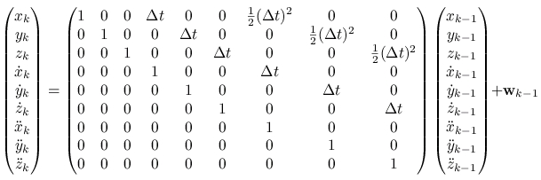
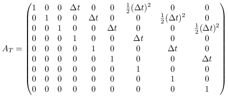
• State Vector: The state vector x is a 9x1 vector containing the positional data (x,y,z) with its first and second derivatives (velocity and acceleration)
  
• Process Model: The process model relates the state at a previous time k-1 with the current state at time k. A is called state transition matrix and w represents the normal distributed process noise with covariance Q. The optional control input Bu is discarded in the second equation.
  
  
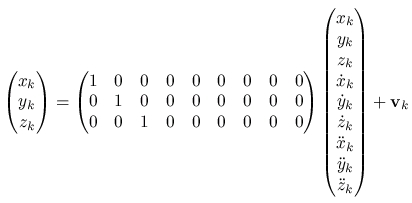
• Measurement Model: The measurement model relates the current state to the measurement z with the matrix H. v is the normal distributed measurement noise with covariance R.
  
  
• Kalman Filter Cycle: The filter equations can be divided in a prediction and a correction step. The prediction step projects forward the current state and covariance to obtain an a priori estimate. After that the correction step uses the incorporates a new measurement to get an improved a posteriori estimate.
  
• Influence of the covariance matrices Q and R
  
  • Q, the process noise covariance, contributes to the overall uncertainty. When Q is large, the Kalman Filter tracks large changes in the data more closely than for smaller Q.
  • R, the measurement noise covariance, determines how much information from the measurement is used. If R is high, the Kalman Filter considers the measurements as not very accurate. For smaller R it will follow the measurements more closely.

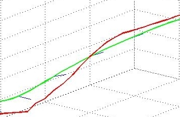
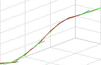
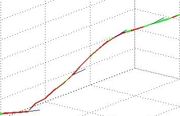
The three images below visualize the positional data. The red lines represent the measurement data, the green lines are the estimated states.

Q small, R large	Q and R equal	Q large, R small

Linear Kalman Filter for the position and orientation tracking

Including orientation as euler angles allows us to keep the linear model from above. The angles can be derived from the quaternion 4-vector by the following formulas.

• State Vector: The state vector x now is expanded. Rotation is added in the form of three euler angles (roll, pitch, jaw) together with their first and second derivatives (angular velocity and acceleration).
  
• Process Model: The process model stays linear and connects position and rotation information of the previous and the next state.
  
  
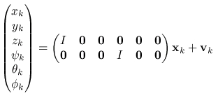
• Measurement Model:
  

Extended Kalman Filter for the position and orientation tracking

As the rotational data is given in the form of quaternions the upper representation is unfavorable. But updating a state vector which contains quaternions requires a non-linear model. Here the extended Kalman Filter can be applied which linearizes about the current mean and covariance.

• State Vector: The rotation entries of the state vector are modified. x now contains the 9 elements for the position, 4 elements of the quaternion and the 6 elements for angular velocity and acceleration as before.
  
• General Process and Measurement Models: The models for the extended Kalman filter are given by the functions f and h.
  
  
• Detailed Process and Measurement Models: The state vector is given as
  
  The function f handles the positional data in the linear way as described above. The quaternion r is updated through a quaternion multiplication with d which represents the difference caused by angular velocity. The angular velocity and acceleration can again be computed linearly.
  The function h has to extract the position (x,y,z) and the quaternion data r from the state vector. For the position this can be done directly, the rotation quaternion needs an additional normalization.
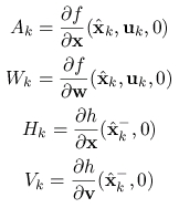
• Kalman Filter Cycle: To take account of the non-linear models the equations for the filter cycle are slightly modified.
  
  The matrices A, H, W, V are Jacobians with partial derivatives of the functions f and h.
  

Fusion of two 6DOF trackers using the Kalman Filter

• Required: HandEyeCalibration to align the two tracker coordinate systems

Fusion of two 6DOF trackers using the federated Kalman Filter

Literature

• R.E. Kalman, A New Approach to Linear Filtering and Prediction Problems, 1960
• A. Gelb (editor), Applied Optimal Estimation
• G. Welch and G. Bishop. An Introduction to the Kalman Filter. Technical Report TR 95-041, University of North Carolina, Department of Computer Science, 1995.
• G. Welch: The Kalman Filter Page
• Neal A Carlson, Federated square root filter for decentralized parallel processors, IEEE Transactions on Aerospace and Electronic Systems, Vol. 26 (3) May 1990, pp. 517-525
• G. Welch: SCAAT: Incremental Tracking with Incomplete Information
• David A. Forsyth, Jean Ponce, Tracking with Linear Dynamic Models, Chapter 17 from "Computer Vision: A Modern Approach"
• D. Pustka: Handling Error in Ubiquitous Tracking Setups^?, diploma thesis, TU Munich, 2004
• Kalman Filtering for Quaternions
• E. W. Weisstein: Quaternions, Mathworld

-- KatharinaPentenrieder - 08 Mar 2005